This is the unpleasant part of data science that makes up around 80% of the work. I recommend skipping to part 3 if you don't have much patience. I'll be using Python and the pandas data analysis library.
The original data can be downloaded from Infochimps.
Cleaning steps
After a lengthy process, I arrive at a dataframe that looks like this:
| state_county | population | num_sightings | raw_rate |
|---|---|---|---|
| alabama autauga | 55246 | 2 | 0.000036 |
| alabama baldwin | 195540 | 32 | 0.000164 |
| alabama barbour | 27076 | 0 | 0.000000 |
| alabama bibb | 22512 | 1 | 0.000044 |
| alabama blount | 57872 | 0 | 0.000000 |
Plotting those raw rates on a map looks like this:
Below are the steps I took:
| step | action | rows remaining |
|---|---|---|
| 1 | convert avro format to pandas DataFrame | 61067 |
| 2 | remove rows with ill-formed dates | 60802 |
| 3 | remove rows before 1990-08-30 | 54444 |
| 4 | remove rows with location outside the contiguous 48 states plus DC | 45983 |
| 5 | make location all uppercase and remove parenthetical comments | 45983 |
| 6 | get county, latitude, longitude from mapquest API | 42998 |
| 7 | convert counties to those used in ggplot2 | 42624 |
| 8 | get county populations from US census data | 42624 |
| 9 | convert the census counties to what's used in ggplot2 | 42624 |
Continue reading if you're interested in the nitty-gritty.
Getting it into a pandas dataframe
The data comes in a few formats, none of which I could get pandas to read correctly. I resorted to using the avro format using a separate library (which required Python 2.x):
#!/usr/bin/python2.7

from avro.datafile import DataFileReader
from avro.io import DatumReader
from pandas import DataFrame

avro_file = '/Users/srharnett/Downloads/ufo_data/ufo_awesome.avro'
reader = DataFileReader(open(avro_file, 'r'), DatumReader())
df = DataFrame(list(reader))
df.to_pickle('ufo_data.pkl')
import numpy as np
import pandas as pd
%load_ext rmagic
%R library(ggplot2)
%R theme_set(theme_bw());
!./convert_data.py
data = pd.read_pickle('ufo_data.pkl')
print(len(data))
data.head()
A couple hundred of the 'sighted_at' dates are 0000, and a dozen or so are pre-1900. A couple others have malformed dates ending in '00'. I remove these rows and convert the strings to a datetime data type.
data = data[[x[-2:] != '00' for x in data.sighted_at]]
data = data[data.sighted_at >= '19000101']
print(len(data))
data.reported_at = pd.to_datetime(data.reported_at)
data.sighted_at = pd.to_datetime(data.sighted_at)
90% of the sightings occurred in the twenty year span 1990-08-30 to 2010-08-30, so I restrict the data to this range. This way we can roughly interpret things as a rate of sightings over time.
%%R -i data -h200
seconds_in_a_year <- 3.15569e7
binwidth <- 5*seconds_in_a_year
ggplot(data, aes(x=sighted_at)) + geom_histogram(binwidth=binwidth)

data.sighted_at.max()
Timestamp('2010-08-30 00:00:00', tz=None)
(data.sighted_at >= '1990-08-30').mean()
0.89543107134633726
data = data[data.sighted_at >= '1990-08-30']
len(data)
54444
Cleaning up the location column
The location column is a bit messy, so I cleaned it up similarly to Machine Learning for Hackers.
# 48 contiguous states plus Washington, D.C.
states = 'AL,AR,AZ,CA,CO,CT,DC,DE,FL,GA,IA,ID,IL,IN,KS,KY,LA,MA,MD,ME,MI,MN,MO,MS,MT,NC,ND,NE,NH,NJ,NM,NV,NY,OH,OK,OR,PA,RI,SC,SD,TN,TX,UT,VA,VT,WA,WI,WV,WY'
states = set(states.split(','))
has_state = np.array([x[-2:].upper() in states for x in data.location])
data = data[has_state]
len(data)
45983
There are a lot of little comments inside parentheses that we'd like to get rid of:
data.location[[x.find('(') >= 0 for x in data.location]].tail()
60885                                Huntsville (near), TX
60890                               Albuquerque (near), NM
60950                             Washington (west of), IA
60975     Laurie (5 mi. W of; 52 mile marker on Osage), MO
61039                                Washington (near), PA
Name: location, dtype: object
import re
pattern = r'(.*)\(.*\)(.*)' # want to ignore anything inside parentheses
r = re.compile(pattern)
def clean_location(loc):
    m = r.search(loc)
    cleaned = m.group(1).strip() + m.group(2).strip() if m is not None else loc.strip()
    return cleaned.upper()
for loc in data.location.tail():
    print('%50s %s %s' % (loc, '-->', clean_location(loc)))
for loc in data.location[[x.find('(') >= 0 for x in data.location]].tail():
    print('%50s %s %s' % (loc, '-->', clean_location(loc)))
data['clean_location'] = [clean_location(x) for x in data.location]
Getting county information -- Mapquest API
Now I'll use the mapquest geocoding API to get county and latitude/longitude information for each location.
import requests
from itertools import zip_longest, islice
MAPQUEST_API_KEY = r'???'
params = dict(key=MAPQUEST_API_KEY, thumbMaps=False)
batch_url = 'http://www.mapquestapi.com/geocoding/v1/batch'

def extract_county(api_result):
    best_guess = api_result['locations'][0]
    location = api_result['providedLocation']['location']
    county = best_guess['adminArea4']
    return location, county

def extract_lat_lng(api_result):
    best_guess = api_result['locations'][0]
    lat, lng = best_guess['latLng']['lat'], best_guess['latLng']['lng']
    return lat, lng

def grouper(iterable, n, fillvalue=None):
    "Collect data into fixed-length chunks or blocks"
    # grouper('ABCDEFG', 3, 'x') --> ABC DEF Gxx
    args = [iter(iterable)] * n
    return zip_longest(fillvalue=fillvalue, *args)

def get_mapquest_results(locations):
    ''' splits up list of locations into chunks of 100 and submits to mapquest API
        returns dictionary location-->county '''
    if MAPQUEST_API_KEY == '???':
        raise ValueError('get your own API key')
    location_to_county = {}
    location_to_latlng = {}
    for chunk in grouper(locations, 100):
        params['location'] = chunk
        r = requests.get(batch_url, params=params)
        for api_result in r.json()['results']:
            location, county = extract_county(api_result)
            lat, lng = extract_lat_lng(api_result)
            location_to_county[location] = county
            location_to_latlng[location] = (lat, lng)
    return location_to_county, location_to_latlng
You'll need a Mapquest API key to actually run this.
location_to_county, location_to_latlng = get_mapquest_results(data.clean_location.head())
import pickle
location_to_county = pickle.load(open('city_to_county.pickle', 'br'))
location_to_latlng = pickle.load(open('coordinates.pickle', 'br'))
for i, (k,v) in enumerate(location_to_county.items()):
    print(k, '|', v)
    if i > 5:
        break
print()
for i, (k,v) in enumerate(location_to_latlng.items()):
    print(k, '|', v)
    if i > 5:
        break
data['latlng'] = [location_to_latlng.get(x) for x in data.clean_location]
data['county'] = [location_to_county.get(x) for x in data.clean_location]
Here I'm dropping rows where Mapquest couldn't find a county, or where the location is outside the contiguous United States.
print(len(data))
data = data[['latlng', 'county', 'clean_location']].dropna()
print(len(data))
data = data[data.county != '']
print(len(data))
data['lat'] = [x[0] for x in data.latlng]
data['lng'] = [x[1] for x in data.latlng]
data = data.query('25.12993 <= lat <= 49.38323 and -124.6813 <= lng <= -67.00742')
print(len(data))
data['state'] = [x[-2:] for x in data.clean_location]
data = data[['lat', 'lng', 'county', 'state']]
data.head()
Map it out, looks similar to the flowingdata and xkcd maps, i.e. simply a map of population density.
%%R -w800 -i data
usa <- map_data("usa")
p <- ggplot(usa, aes(x=long, y=lat))
p <- p + geom_polygon(alpha=.1)
p <- p + geom_point(aes(x=lng, y=lat), data=data, alpha=.01, color='blue', size=3)
p + coord_map("conic", lat0=30)

Binning by county
To bin by county, I'm going to use the US county map from ggplot. Unfortunately the county names from the mapquest API don't match these exactly, so we're going to have to do a little more munging.
%%R -o county_sightings
county_sightings <- map_data("county")
head(county_sightings)
       long      lat group order  region subregion
1 -86.50517 32.34920     1     1 alabama   autauga
2 -86.53382 32.35493     1     2 alabama   autauga
3 -86.54527 32.36639     1     3 alabama   autauga
4 -86.55673 32.37785     1     4 alabama   autauga
5 -86.57966 32.38357     1     5 alabama   autauga
6 -86.59111 32.37785     1     6 alabama   autauga
county_sightings = DataFrame(dict(state=county_sightings[4], county=county_sightings[5]))
county_sightings['num_sightings'] = 0
county_sightings = county_sightings.drop_duplicates().set_index(['state', 'county'])
county_sightings.head()
Our data uses the state abbreviations (e.g. AL for alabama) so we'll need to convert these.
state_map = {'alabama': 'AL', 'arizona': 'AZ', 'arkansas': 'AR', 'california': 'CA', 'colorado': 'CO',
       'connecticut': 'CT', 'delaware': 'DE', 'district of columbia': 'DC', 'florida': 'FL',
       'georgia': 'GA', 'idaho': 'ID', 'illinois': 'IL', 'indiana': 'IN', 'iowa': 'IA', 'kansas': 'KS',
       'kentucky': 'KY', 'louisiana': 'LA', 'maine': 'ME', 'maryland': 'MD', 'massachusetts': 'MA',
       'michigan': 'MI', 'minnesota': 'MN', 'mississippi': 'MS', 'missouri': 'MO', 'montana': 'MT',
       'nebraska': 'NE', 'nevada': 'NV', 'new hampshire': 'NH', 'new jersey': 'NJ', 'new mexico': 'NM',
       'new york': 'NY', 'north carolina': 'NC', 'north dakota': 'ND', 'ohio': 'OH', 'oklahoma': 'OK',
       'oregon': 'OR', 'pennsylvania': 'PA', 'rhode island': 'RI', 'south carolina': 'SC',
       'south dakota': 'SD', 'tennessee': 'TN', 'texas': 'TX', 'utah': 'UT', 'vermont': 'VT', 'virginia': 'VA',
       'washington': 'WA', 'west virginia': 'WV', 'wisconsin': 'WI', 'wyoming': 'WY'}
state_map_rev = {v: k for k,v in state_map.items()}
from collections import defaultdict, Counter
The mapping of counties in our data set to the ggplot ones is a pretty painful manual process. I gave up after getting the majority of them.
%%time
missing_counties = defaultdict(Counter) # counties that failed to map to a county in the ggplot set

def convert_to_ggplot_style(x):
    ''' takes a row from our main dataframe 'data' and updates the appropriate county in the new dataframe
        'county_sightings' if it can find the county, otherwise updates missing_counties '''
    state = state_map_rev[x['state']]
    county = x['county'].lower().replace("'", '').replace('.', '')
    if county.split()[-1] in {'county', 'parish'}:
        county = county[:-7]
    known_fixes = {'dupage': 'du page',
                   'district of columbia': 'washington',
                   'desoto': 'de soto',
                   'dekalb': 'de kalb'}
    county = known_fixes.get(county, county)
    try:
        county_sightings.ix[state, county] += 1
    except KeyError:
        missing_counties[state][county] += 1
data.apply(convert_to_ggplot_style, axis=1)
print(county_sightings.head())
We could add more to the 'known fixes' dictionary to get more of these, but there aren't too many and Virginia is a little weird when it comes to counties.
# number of sightings lost in the conversion
sum(count for counter in missing_counties.values() for count in counter.values())
374
for state, counter in missing_counties.items():
    for county, count in counter.most_common():
        if count >= 6:
            print(state, county, count)
county_sightings = county_sightings.reset_index()
county_sightings['state_county'] = county_sightings.apply(lambda x: x.state + ' ' + x.county, axis=1)
county_sightings = county_sightings[['state_county', 'num_sightings']]
county_sightings.head()
county_sightings.num_sightings.sum()
42624
Counties in the west are larger, so this doesn't quite look the same as the flowing data and xkcd maps.
%%R -i county_sightings -w900
counties <- map_data("county")
counties$region <- do.call(paste, c(counties[c("region", "subregion")], sep = " "))

p <- ggplot(county_sightings, aes(map_id=state_county))
p <- p + geom_map(aes(fill=num_sightings), map=counties)
p <- p + expand_limits(x=counties$long, y=counties$lat)
p <- p + coord_map("conic", lat0=30) + scale_fill_gradientn(trans="sqrt", colours=c('white', '#640000'))
p + ggtitle('UFO sightings by county') + xlab('long') + ylab('lat')

Get county populations from census data
I used a data set found here:
http://www.census.gov/popest/data/counties/totals/2013/CO-EST2013-alldata.html
populations = pd.read_csv('CO-EST2013-Alldata.csv', encoding='ISO-8859-1')
populations.head()
county_populations = populations.query('SUMLEV == 50')[['STNAME', 'CTYNAME', 'POPESTIMATE2013']]
county_populations.columns = ['state', 'county', 'population']
county_populations.state = [x.lower() for x in county_populations.state]
county_populations.county = [x.lower().replace("'", '').replace('.', '') for x in county_populations.county]
county_populations.head()
And now again, the painful process of converting this to the ggplot states and counties.
def convert_to_ggplot_style(x):
    state = x.state
    county = x.county
    if county.split()[-1] in {'county', 'parish'}:
        county = county[:-7]
    if county.split()[-1] == 'city':
        county = county[:-5]
    known_fixes = {'dupage': 'du page',
                   'district of columbia': 'washington',
                   'desoto': 'de soto',
                   'dekalb': 'de kalb',
                   'lasalle': 'la salle',
                   'laporte': 'la porte',
                   'dewitt': 'de witt',
                   'lamoure': 'la moure',
                   'doña ana': 'dona ana'}
    county = known_fixes.get(county, county)
    if state == 'nevada' and county == 'carson':
        county = 'carson city'
    return county
county_populations.county = county_populations.apply(convert_to_ggplot_style, axis=1)
county_populations['state_county'] = county_populations.apply(lambda x: x.state + ' ' + x.county, axis=1)
county_populations = county_populations[['state_county', 'population']]
county_populations.head()
Counties in Alaska and Hawaii, as well as some in Virginia, are in the population data but not the filtered UFO sighting data. There's also a couple where there's a city and county with the same name, so I'll combine those.
print(len(county_populations), len(county_populations.state_county.unique()))
county_populations = county_populations.groupby('state_county').sum().reset_index()
print(len(county_populations))
county_populations.head()
final_data = pd.merge(county_populations, county_sightings, on='state_county', how='left')
print(len(county_populations), len(county_sightings), len(final_data))
final_data = final_data.fillna(0)
final_data.head()
final_data.num_sightings.sum()
42624.0
final_data.to_csv('ufo_data.csv')
I've made this cleaned up data available here
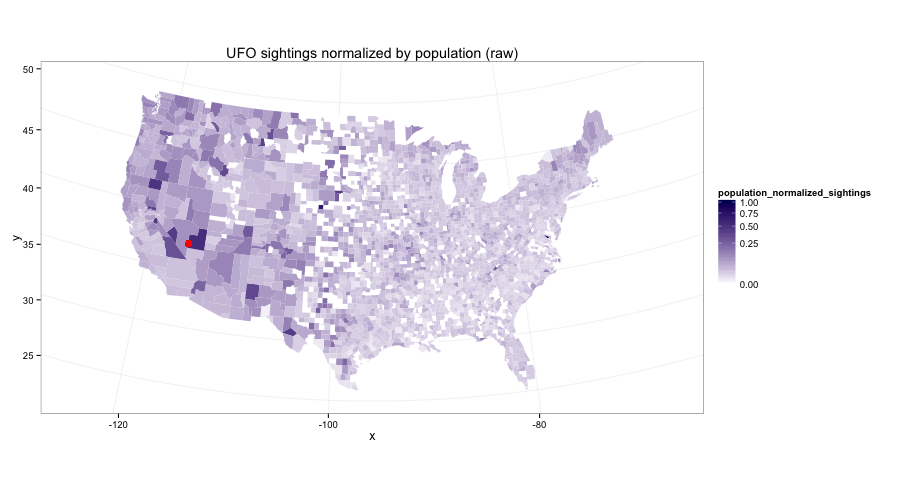
UFO sightings normalized by population, raw
Finally, a first answer to the original question.
final_data.eval('raw_rate = num_sightings/population')
%%R -i final_data -w900
counties <- map_data("county")
counties$region <- do.call(paste, c(counties[c("region", "subregion")], sep = " "))

p <- ggplot(final_data, aes(map_id=state_county))
p <- p + geom_map(aes(fill=raw_rate), map=counties)
p <- p + expand_limits(x=counties$long, y=counties$lat)
p <- p + coord_map("conic", lat0=30) + scale_fill_gradientn(trans="sqrt", colours=c('white', '#640000'))
p + ggtitle('UFO sightings adjusted for population (raw)') + xlab('long') + ylab('lat')

In part 3 I explore a few ways to smooth this out so that the county-level estimates are more reasonable.
!date